Diebold-Mariano test¶

This module provides a function DM that implements the one-sided version of the Diebold-Mariano (DM) test in the context of electricity price forecasting.

Besides the DM test, the module also provides a function plot_multivariate_DM_test to plot the DM results when comparing multiple forecasts.

DM test¶

The Diebold-Mariano (DM) test is probably the most commonly used tool to evaluate the significance of differences in forecasting accuracy. It is an asymptotic z-test of the hypothesis that the mean of the loss differential series:

\[\begin{equation} \Delta^{\mathrm{A, B}}_{k} = L(\varepsilon^\mathrm{A}_{k}) - L(\varepsilon^\mathrm{B}_{k}) \end{equation}\]

where \(\varepsilon^\mathrm{Z}_{k}=p_{k}-\hat{p}_{k}\) is the prediction error of model Z for time step \(k\) and \(L(\cdot)\) is the loss function. For point forecasts, we usually take \(L(\varepsilon^\mathrm{Z}_{k})=|\varepsilon^\mathrm{Z}_{k}|^p\) with \(p=1\) or \(2\), which corresponds to the absolute and squared losses.

This module implements the one-sided version of the DM test using the a function DM function. Given the forecast of a model A and the forecast of a model B, the test evaluates the null hypothesis \(H_0\) of the mean of the loss differential of model A being lower or equal than that of model B. Hence, rejecting the null \(H_0\) means that the forecasts of model B are significantly more accurate than those of model A.

The module provides the two standard versions of the test in electricity price forecasting: an univariate and a multivariate version. The univariate version of the test has the advantage of providing a deeper analysis as it indicates which forecast is significantly better for which hour of the days. The multivariate version grants a better representation of the results as it summarizes the comparison in a single p-value.

epftoolbox.evaluation.DM(p_real, p_pred_1, p_pred_2, norm=1, version='univariate')[source]¶

Function that performs the one-sided DM test in the contex of electricity price forecasting

The test compares whether there is a difference in predictive accuracy between two forecast p_pred_1 and p_pred_2. Particularly, the one-sided DM test evaluates the null hypothesis H0 of the forecasting errors of p_pred_2 being larger (worse) than the forecasting errors p_pred_1 vs the alternative hypothesis H1 of the errors of p_pred_2 being smaller (better). Hence, rejecting H0 means that the forecast p_pred_2 is significantly more accurate that forecast p_pred_1. (Note that this is an informal definition. For a formal one we refer to here)

Two versions of the test are possible:

1. A univariate version with as many independent tests performed as prices per day, i.e. 24 tests in most day-ahead electricity markets.

2. A multivariate with the test performed jointly for all hours using the multivariate loss differential series (see this article for details.

Parameters:	p_real (numpy.ndarray) – Array of shape \((n_\mathrm{days}, n_\mathrm{prices/day})\) representing the real market prices p_pred_1 (TYPE) – Array of shape \((n_\mathrm{days}, n_\mathrm{prices/day})\) representing the first forecast p_pred_2 (TYPE) – Array of shape \((n_\mathrm{days}, n_\mathrm{prices/day})\) representing the second forecast norm (int, optional) – Norm used to compute the loss differential series. At the moment, this value must either be 1 (for the norm-1) or 2 (for the norm-2). version (str, optional) – Version of the test as defined in here. It can have two values: `'univariate` or `'multivariate`
Returns:	The p-value after performing the test. It is a float in the case of the multivariate test and a numpy array with a p-value per hour for the univariate test
Return type:	float, numpy.ndarray

Example

>>> from epftoolbox.evaluation import DM
>>> from epftoolbox.data import read_data
>>> import pandas as pd
>>>
>>> # Generating forecasts of multiple models
>>>
>>> # Download available forecast of the NP market available in the library repository
>>> # These forecasts accompany the original paper
>>> forecasts = pd.read_csv('https://raw.githubusercontent.com/jeslago/epftoolbox/master/' +
...                       'forecasts/Forecasts_NP_DNN_LEAR_ensembles.csv', index_col=0)
>>>
>>> # Deleting the real price field as it the actual real price and not a forecast
>>> del forecasts['Real price']
>>>
>>> # Transforming indices to datetime format
>>> forecasts.index = pd.to_datetime(forecasts.index)
>>>
>>> # Extracting the real prices from the market
>>> _, df_test = read_data(path='.', dataset='NP', begin_test_date=forecasts.index[0],
...                        end_test_date=forecasts.index[-1])
Test datasets: 2016-12-27 00:00:00 - 2018-12-24 23:00:00
>>>
>>> real_price = df_test.loc[:, ['Price']]
>>>
>>> # Testing the univariate DM version on an ensemble of DNN models versus an ensemble
>>> # of LEAR models
>>> DM(p_real=real_price.values.reshape(-1, 24),
...     p_pred_1=forecasts.loc[:, 'LEAR Ensemble'].values.reshape(-1, 24),
...     p_pred_2=forecasts.loc[:, 'DNN Ensemble'].values.reshape(-1, 24),
...     norm=1, version='univariate')
array([9.99999944e-01, 9.97562415e-01, 8.10333949e-01, 8.85201928e-01,
       9.33505978e-01, 8.78116764e-01, 1.70135981e-02, 2.37961920e-04,
       5.52337353e-04, 6.07843340e-05, 1.51249750e-03, 1.70415008e-03,
       4.22319907e-03, 2.32808010e-03, 3.55958698e-03, 4.80663621e-03,
       1.64841032e-04, 4.55829140e-02, 5.86609688e-02, 1.98878375e-03,
       1.04045731e-01, 8.71203187e-02, 2.64266732e-01, 4.06676195e-02])
>>>
>>> # Testing the multivariate DM version
>>> DM(p_real=real_price.values.reshape(-1, 24),
...     p_pred_1=forecasts.loc[:, 'LEAR Ensemble'].values.reshape(-1, 24),
...     p_pred_2=forecasts.loc[:, 'DNN Ensemble'].values.reshape(-1, 24),
...     norm=1, version='multivariate')
0.003005725748326471

plot_multivariate_DM_test¶

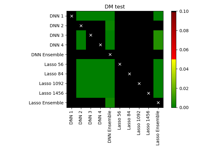
The plot_multivariate_DM_test provides an easy-to-use interface to plot in a heat map with a chessboard shape the results of using the DM test to compare the forecasts of multiple models. An example of the heat map is provided below in the function example.

epftoolbox.evaluation.plot_multivariate_DM_test(real_price, forecasts, norm=1, title='DM test', savefig=False, path='')[source]¶

Plotting the results of comparing forecasts using the multivariate DM test.

The resulting plot is a heat map in a chessboard shape. It represents the p-value of the null hypothesis of the forecast in the y-axis being significantly more accurate than the forecast in the x-axis. In other words, p-values close to 0 represent cases where the forecast in the x-axis is significantly more accurate than the forecast in the y-axis.

Parameters:

real_price (pandas.DataFrame) – Dataframe that contains the real prices
forecasts (TYPE) – Dataframe that contains the forecasts of different models. The column names are the forecast/model names. The number of datapoints should equal the number of datapoints in real_price.
norm (int, optional) – Norm used to compute the loss differential series. At the moment, this value must either be 1 (for the norm-1) or 2 (for the norm-2).
title (str, optional) – Title of the generated plot
savefig (bool, optional) – Boolean that selects whether the figure should be saved in the current folder
path (str, optional) – Path to save the figure. Only necessary when savefig=True

Example

>>> from epftoolbox.evaluation import DM, plot_multivariate_DM_test
>>> from epftoolbox.data import read_data
>>> import pandas as pd
>>>
>>> # Generating forecasts of multiple models
>>>
>>> # Download available forecast of the NP market available in the library repository
>>> # These forecasts accompany the original paper
>>> forecasts = pd.read_csv('https://raw.githubusercontent.com/jeslago/epftoolbox/master/' +
...                       'forecasts/Forecasts_NP_DNN_LEAR_ensembles.csv', index_col=0)
>>>
>>> # Deleting the real price field as it the actual real price and not a forecast
>>> del forecasts['Real price']
>>>
>>> # Transforming indices to datetime format
>>> forecasts.index = pd.to_datetime(forecasts.index)
>>>
>>> # Extracting the real prices from the market
>>> _, df_test = read_data(path='.', dataset='NP', begin_test_date=forecasts.index[0],
...                        end_test_date=forecasts.index[-1])
Test datasets: 2016-12-27 00:00:00 - 2018-12-24 23:00:00
>>>
>>> real_price = df_test.loc[:, ['Price']]
>>>
>>> # Generating a plot to compare the models using the multivariate DM test
>>> plot_multivariate_DM_test(real_price=real_price, forecasts=forecasts)