Giacomini-White test
This module provides a function GW that implements the one-sided version of the Giacomini-White (GW) test for Conditional Predictive Ability (CPA) in the context of electricity price forecasting.
Additionally, the module provides a function plot_multivariate_GW_test that plots the results of pairwise comparisonsi between multiple models.
GW test
The Giacomini-White (GW) test can be seen as a generalization of the Diebold-Mariano test that measures the CPA instead of the Unconditional Predictive Ability. The test, like the DM variant, measures the statistical significance of the differences of two models forecasts. It is an asymptotic \(\chi^2\)-test of the null hypothesis \(\mathrm{H}_0:\phi=0\) in the regression:
where \(\mathbb{X}_{d-1}\) contains elements from the information set on day \(d-1\), i.e., a constant and lags of \(\Delta^{\mathrm{A, B}}_d\). The loss differential is obtained like in the DM test:
where \(\varepsilon^\mathrm{Z}_{k}=p_{k}-\hat{p}_{k}\) is the prediction error of model Z for time step \(k\) and \(L(\cdot)\) is the loss function. For point forecasts, we usually take \(L(\varepsilon^\mathrm{Z}_{k})=|\varepsilon^\mathrm{Z}_{k}|^p\) with \(p=1\) or \(2\), which corresponds to the absolute and squared losses.
This module implements the one-sided version of the GW test using the a function GW function. Given the forecast of a model A and the forecast of a model B, the test evaluates the null hypothesis \(H_0\) of the CPA of the loss differential of model A being higher or equal than that of model B. Hence, rejecting the null \(H_0\) means that the forecasts of model B are significantly more accurate than those of model A.
The module provides the two standard versions of the test in electricity price forecasting: an univariate and a multivariate version. The univariate version of the test has the advantage of providing a deeper analysis as it indicates which forecast is significantly better for which hour of the days. The multivariate version grants a better representation of the results as it summarizes the comparison in a single p-value.
-
epftoolbox.evaluation.GW(p_real, p_pred_1, p_pred_2, norm=1, version='univariate')[source]¶ Perform the one-sided GW test
The test compares the Conditional Predictive Accuracy of two forecasts
p_pred_1andp_pred_2. The null H0 is that the CPA of errorsp_pred_1is higher (better) or equal to the errors ofp_pred_2vs. the alternative H1 that the CPA ofp_pred_2is higher. Rejecting H0 means that the forecastsp_pred_2are significantly more accurate than forecastsp_pred_1. (Note that this is an informal definition. For a formal one we refer here)Parameters: - p_real (numpy.ndarray) – Array of shape \((n_\mathrm{days}, n_\mathrm{prices/day})\) representing the real market prices
- p_pred_1 (TYPE) – Array of shape \((n_\mathrm{days}, n_\mathrm{prices/day})\) representing the first forecast
- p_pred_2 (TYPE) – Array of shape \((n_\mathrm{days}, n_\mathrm{prices/day})\) representing the second forecast
- norm (int, optional) – Norm used to compute the loss differential series. At the moment, this value must either be 1 (for the norm-1) or 2 (for the norm-2).
- version (str, optional) –
Version of the test as defined in here. It can have two values:
'univariate'or'multivariate'
Returns: The p-value after performing the test. It is a float in the case of the multivariate test and a numpy array with a p-value per hour for the univariate test
Return type: float, numpy.ndarray
Example
>>> from epftoolbox.evaluation import GW
>>> from epftoolbox.data import read_data
>>> import pandas as pd
>>>
>>> # Generating forecasts of multiple models
>>>
>>> # Download available forecast of the NP market available in the library repository
>>> # These forecasts accompany the original paper
>>> forecasts = pd.read_csv('https://raw.githubusercontent.com/jeslago/epftoolbox/master/' +
...                       'forecasts/Forecasts_NP_DNN_LEAR_ensembles.csv', index_col=0)
>>>
>>> # Deleting the real price field as it the actual real price and not a forecast
>>> del forecasts['Real price']
>>>
>>> # Transforming indices to datetime format
>>> forecasts.index = pd.to_datetime(forecasts.index)
>>>
>>> # Extracting the real prices from the market
>>> _, df_test = read_data(path='.', dataset='NP', begin_test_date=forecasts.index[0],
...                        end_test_date=forecasts.index[-1])
Test datasets: 2016-12-27 00:00:00 - 2018-12-24 23:00:00
>>>
>>> real_price = df_test.loc[:, ['Price']]
>>>
>>> # Testing the univariate GW version on an ensemble of DNN models versus an ensemble
>>> # of LEAR models
>>> GW(p_real=real_price.values.reshape(-1, 24),
...     p_pred_1=forecasts.loc[:, 'LEAR Ensemble'].values.reshape(-1, 24),
...     p_pred_2=forecasts.loc[:, 'DNN Ensemble'].values.reshape(-1, 24),
...     norm=1, version='univariate')
array([1.00000000e+00, 1.00000000e+00, 1.00000000e+00, 1.00000000e+00,
       1.00000000e+00, 1.00000000e+00, 1.03217562e-01, 2.63206239e-03,
       5.23325510e-03, 5.90845414e-04, 6.55116487e-03, 9.85034605e-03,
       3.34250412e-02, 1.80798591e-02, 2.74761848e-02, 3.19436776e-02,
       8.39512169e-04, 2.11907847e-01, 5.79718600e-02, 8.73956638e-03,
       4.30521699e-01, 2.67395381e-01, 6.33448562e-01, 1.99826993e-01])
>>>
>>> # Testing the multivariate GW version
>>> GW(p_real=real_price.values.reshape(-1, 24),
...     p_pred_1=forecasts.loc[:, 'LEAR Ensemble'].values.reshape(-1, 24),
...     p_pred_2=forecasts.loc[:, 'DNN Ensemble'].values.reshape(-1, 24),
...     norm=1, version='multivariate')
0.017598166936843906
plot_multivariate_GW_test
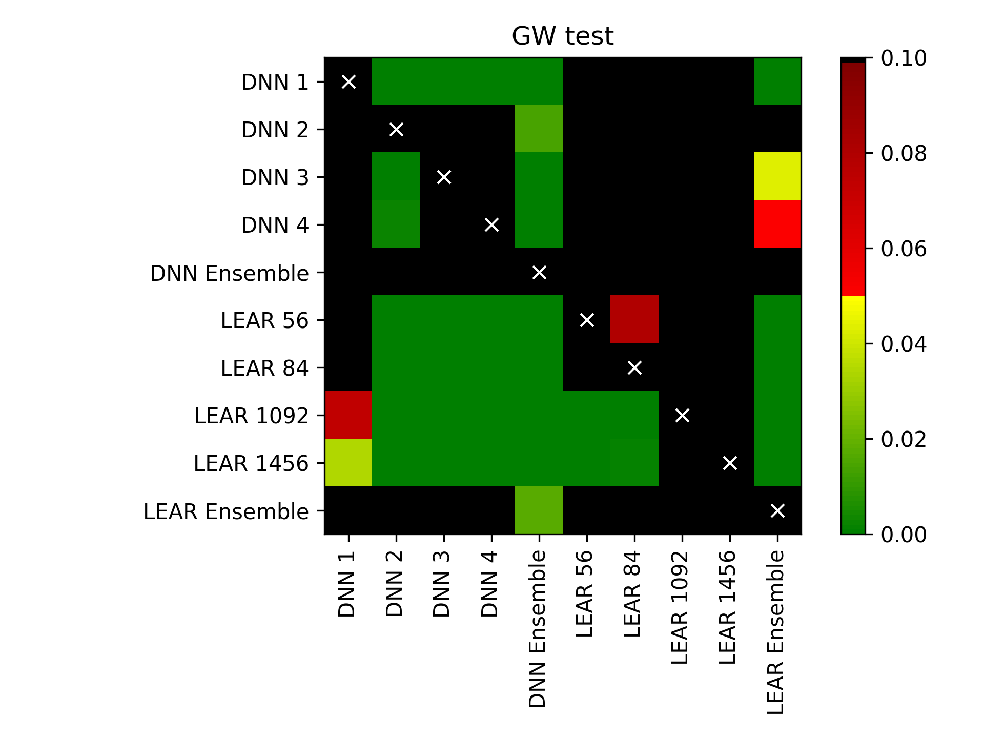
The plot_multivariate_GW_test provides an easy-to-use interface to plot in a heat map with a chessboard shape the results of using the DM test to compare the forecasts of multiple models. An example of the heat map is provided below in the function example.
-
epftoolbox.evaluation.plot_multivariate_GW_test(real_price, forecasts, norm=1, title='GW test', savefig=False, path='')[source]¶ Plotting the results of comparing forecasts using the multivariate GW test.
The resulting plot is a heat map in a chessboard shape. It represents the p-value of the null hypothesis of the forecast in the y-axis being significantly more accurate than the forecast in the x-axis. In other words, p-values close to 0 represent cases where the forecast in the x-axis is significantly more accurate than the forecast in the y-axis.
Parameters: - real_price (pandas.DataFrame) – Dataframe that contains the real prices
- forecasts (TYPE) – Dataframe that contains the forecasts of different models. The column names are the
forecast/model names. The number of datapoints should equal the number of datapoints
in
real_price. - norm (int, optional) – Norm used to compute the loss differential series. At the moment, this value must either be 1 (for the norm-1) or 2 (for the norm-2).
- title (str, optional) – Title of the generated plot
- savefig (bool, optional) – Boolean that selects whether the figure should be saved in the current folder
- path (str, optional) – Path to save the figure. Only necessary when savefig=True
Example
>>> from epftoolbox.evaluation import GW, plot_multivariate_GW_test
>>> from epftoolbox.data import read_data
>>> import pandas as pd
>>>
>>> # Generating forecasts of multiple models
>>>
>>> # Download available forecast of the NP market available in the library repository
>>> # These forecasts accompany the original paper
>>> forecasts = pd.read_csv('https://raw.githubusercontent.com/jeslago/epftoolbox/master/' +
...                       'forecasts/Forecasts_NP_DNN_LEAR_ensembles.csv', index_col=0)
>>>
>>> # Deleting the real price field as it the actual real price and not a forecast
>>> del forecasts['Real price']
>>>
>>> # Transforming indices to datetime format
>>> forecasts.index = pd.to_datetime(forecasts.index)
>>>
>>> # Extracting the real prices from the market
>>> _, df_test = read_data(path='.', dataset='NP', begin_test_date=forecasts.index[0],
...                        end_test_date=forecasts.index[-1])
Test datasets: 2016-12-27 00:00:00 - 2018-12-24 23:00:00
>>>
>>> real_price = df_test.loc[:, ['Price']]
>>>
>>> # Generating a plot to compare the models using the multivariate GW test
>>> plot_multivariate_GW_test(real_price=real_price, forecasts=forecasts)